Designing Dynamic Experiments
The formal definition of the Design of Dynamic Experiment (DoDE) has been described in this 2013 publication. Here we describe the methodology by a very simple example: a reaction network taking place in a batch reactor. We do not have a detailed kinetic model for such a reaction, but we have some partial stoichiometric information and, from thermodynamics, we estimate that the main reaction is endothermic. We know that the two reactants A and B react to produce C through this reaction: A+2B↔C. However, there is an undesirable byproduct D that we wish to minimize. We do not know if the byproduct D is formed directly from A, B or C through one of the following reactions: C→D+E, A→D+F, or B→D or some other way. Our stoichiometric knowledge is partial.
Because we do not have a detailed knowledge-driven model, we cannot calculate the optimal temperature profile, which will result in the largest amount of desired product C, while the undesired D is kept below a threshold concentration. Thus, we resort to experiments in which different temperature profiles are tried. We hope that the results of the experiments will lead us to a data-driven model through which the optimal time-dependent temperature profile with time will be selected. Clearly, we need to systematically choose the temperature profiles with time to examine all possibilities. However, we desire to do the minimum number of experiments. This is what is accomplished with the DoDE methodology.
The key innovative idea that gave birth to the DoDE methodology was the parametrization of the temperature profile as a linear combination of shifted Legendre polynomials which are orthogonal in the (0, 1) interval.

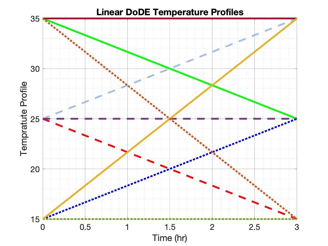
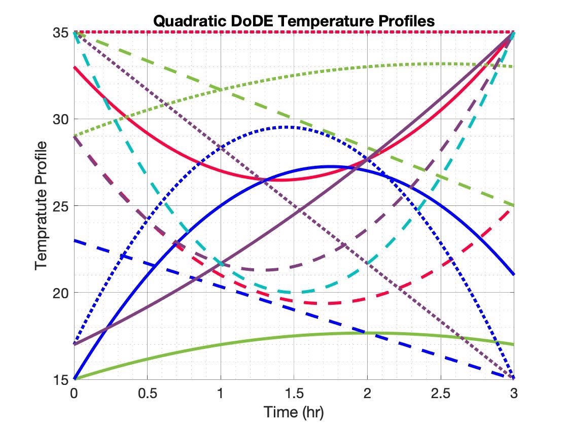
Here the reactor temperature ranges between 15 and 35 °C. One has now to decide how many polynomials to use and select the values of the x1, x2, etc. variables in each experiment. These variables are called dynamic subfactors. As the number of polynomials used to parametrize the temperature profile increases, so do the number of dynamic subfactors. This implies an even larger increase in the number of experiments.


If one starts with the set of experiments in Figure 1, some additional experiments like those in Figure 2 can be appended later a second cycle of experimentation to also explore quadratic profiles of the temperature dependence on time. For more details on the Design of Dynamic Experiments (DoDE) methodology, please consult our publications here.
